Note
Click here to download the full example code
Duffing
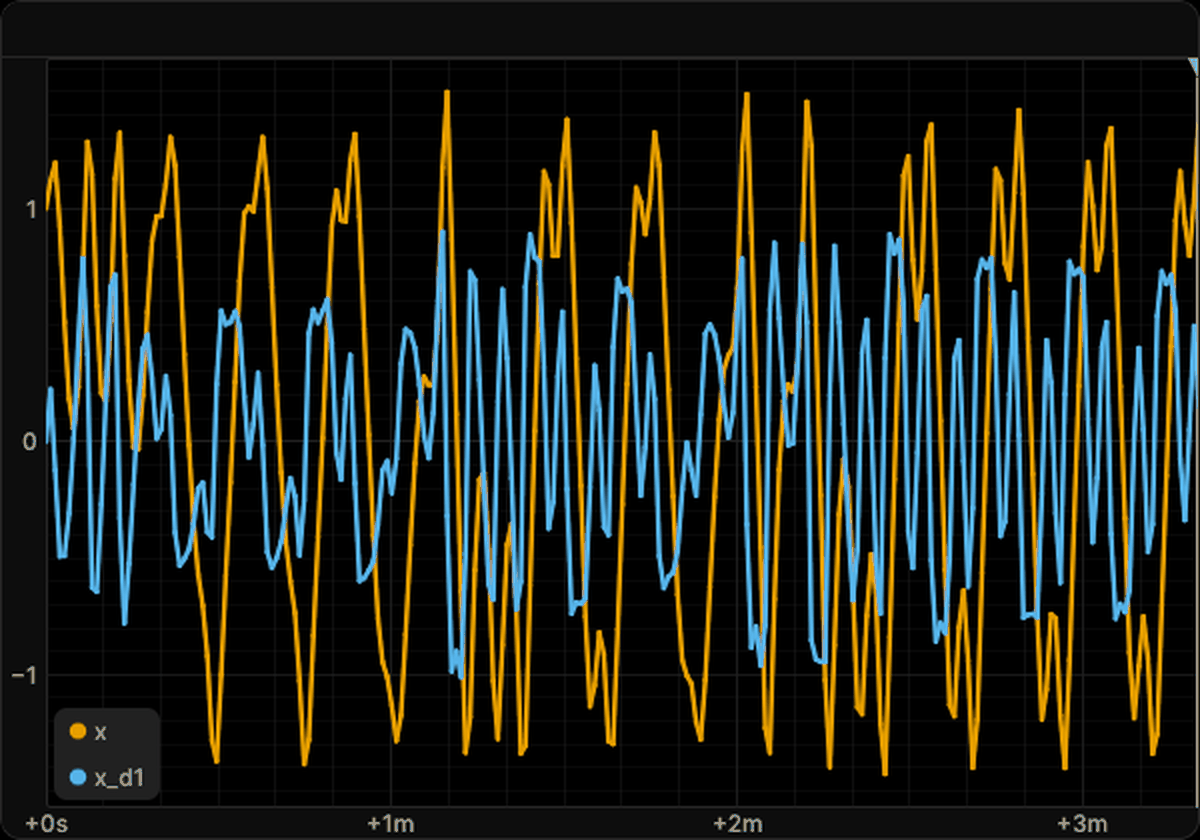
A forced, damped particle in a double-well potential never settles: it hops irregularly between the two wells at
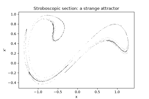
x = -1 and x = 1, and the stroboscopic picture of its motion is a folded strange attractor.
The parameters are the classic chaotic ones, delta = 0.3, alpha = -1, beta = 1, gamma = 0.5,
omega = 1.2. The default blueprint shows the position and the velocity as time series over the whole run of about
forty forcing periods.
import math

import matplotlib.pyplot as plt

from skcomplex.analysis import SectionAnalysis
from skcomplex.engine.runtime import Simulation
from skcomplex.engine.viz import RerunObserver
from skcomplex.models import create

MODEL = 'duffing'

system = create(MODEL)
observer = RerunObserver(MODEL, save_path=f'{MODEL}.rrd', blueprint='default', interval=16)
simulation = Simulation(system, dt=0.05, observers=[observer]).check().prepare().run(until=200)
Open the recording in the Rerun viewer
Stroboscopic section
Sampling the state once per forcing period 2π / ω removes the drive from the picture. A periodic response would
leave a few isolated points, while the chaotic Duffing oscillator should fill a folded, layered set, Ueda's strange
attractor, with points in both wells.
section = SectionAnalysis('stroboscopic', period=2 * math.pi / 1.2, n_points=3000, transient=50)
section.check().prepare(create(MODEL)).run()
fig, ax = plt.subplots(figsize=(6, 4))
ax.plot(section.values_['duffing.x'], section.values_['duffing.x_d1'], ',', color='black', alpha=0.6)
ax.set_xlabel('x')
ax.set_ylabel("x'")
ax.set_title('Stroboscopic section: a strange attractor')
plt.show()
About the model
The forced Duffing oscillator x'' = -delta x' - alpha x - beta x^3 + gamma cos(omega t), chaotic here.
References
- Duffing 1918
- Trzaska 2023
Total running time of the script: ( 0 minutes 25.690 seconds)
Download Python source code: plot_duffing.py