Note
Click here to download the full example code
Geometric Brownian motion
The price of an asset follows dS = mu S dt + sigma S dW, the model behind Black and Scholes' option pricing. The
returns are proportional to the price, so the price stays positive and wanders on a logarithmic scale, and the
log-price is a Brownian motion with drift mu - sigma^2 / 2.
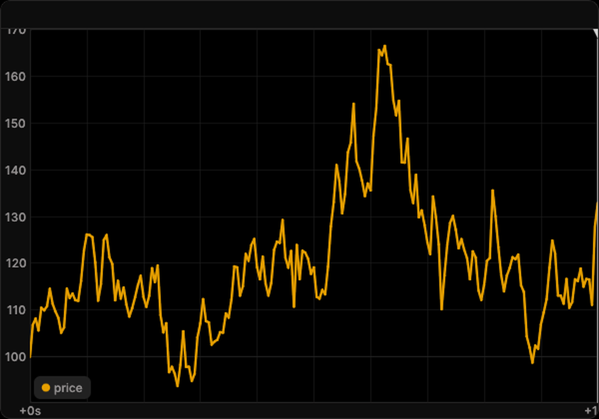
The price starts at 100 with a drift of 5 percent and a volatility of 20 percent a year, and is simulated for ten years in steps of 0.05. The default blueprint shows one path of the price.
import matplotlib.pyplot as plt
import numpy as np
from scipy import stats

from skcomplex.engine.runtime import Simulation
from skcomplex.engine.viz import RerunObserver
from skcomplex.models import create

MODEL = 'geometric_brownian_motion'
PRICE, MU, SIGMA, YEARS, DT = 100.0, 0.05, 0.2, 10, 0.05

observer = RerunObserver(MODEL, save_path=f'{MODEL}.rrd', blueprint='default', interval=1)
system = create(MODEL, price=PRICE, mu=MU, sigma=SIGMA)
simulation = Simulation(system, dt=DT, observers=[observer], random_state=0).check().prepare().run(until=YEARS)
Open the recording in the Rerun viewer
Log returns
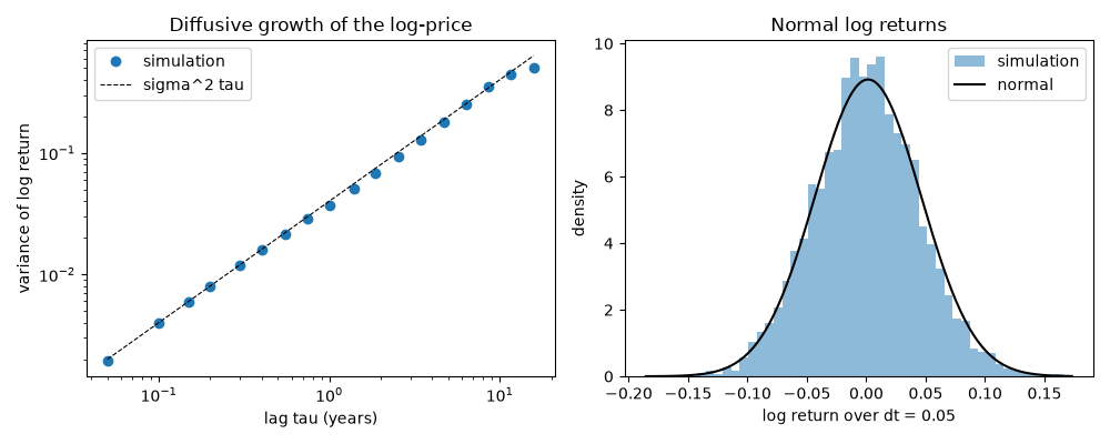
The log returns over a lag tau are independent and normal with mean (mu - sigma^2 / 2) tau and variance
sigma^2 tau. Along one path of 200 years, the variance of the log returns should grow linearly with the lag, and
the one-step log returns should follow that normal density.
long_run = (
    Simulation(create(MODEL, price=PRICE, mu=MU, sigma=SIGMA), dt=DT, random_state=1).check().prepare().run(until=200)
)
logs = np.log(long_run.trajectory_.values('asset.price'))
lags = np.unique(np.logspace(0, 2.5, 20).astype(int))
returns = logs[1:] - logs[:-1]
grid = np.linspace(returns.min(), returns.max(), 200)
fig, (scaling, density) = plt.subplots(1, 2, figsize=(10, 4))
scaling.loglog(lags * DT, [np.var(logs[lag:] - logs[:-lag]) for lag in lags], 'o', label='simulation')
scaling.loglog(lags * DT, SIGMA**2 * lags * DT, 'k--', lw=0.8, label='sigma^2 tau')
scaling.set_xlabel('lag tau (years)')
scaling.set_ylabel('variance of log return')
scaling.set_title('Diffusive growth of the log-price')
scaling.legend()
density.hist(returns, bins=50, density=True, alpha=0.5, label='simulation')
mean, std = (MU - SIGMA**2 / 2) * DT, SIGMA * np.sqrt(DT)
density.plot(grid, stats.norm.pdf(grid, mean, std), 'k', label='normal')
density.set_xlabel(f'log return over dt = {DT}')
density.set_ylabel('density')
density.set_title('Normal log returns')
density.legend()
fig.tight_layout()
plt.show()
About the model
An asset whose price follows geometric Brownian motion.
References
- Black and Scholes 1973
Total running time of the script: ( 0 minutes 6.032 seconds)
Download Python source code: plot_geometric_brownian_motion.py
Download Jupyter notebook: plot_geometric_brownian_motion.ipynb