Note

Click here to download the full example code

Correlated geometric Brownian motions

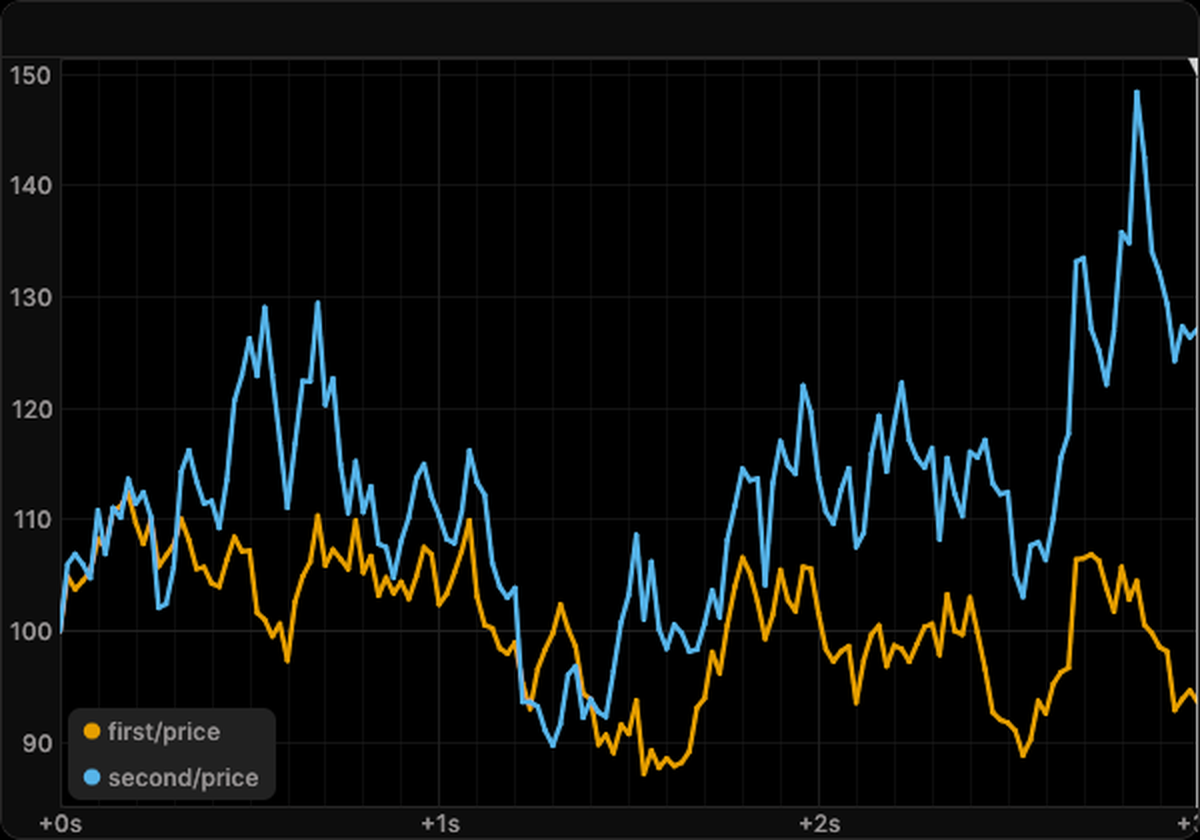
Two asset prices follow geometric Brownian motions driven by the two processes of one WienerProcess, whose covariance gives them the correlation rho = 0.7. The prices wander apart on their own drifts and volatilities, but they rise and fall together, and their log returns are correlated with rho.

The model is created by name from the catalog with prices of 100, drifts of 5 and 8 percent, and volatilities of 20 and 30 percent a year. It is simulated for three years in frames of 0.02 with the Euler-Maruyama scheme. The default blueprint shows both prices in one time series view. The WienerProcess that both motions bind is no component and draws no view.

import matplotlib.pyplot as plt
import numpy as np

from skcomplex.engine.runtime import Simulation
from skcomplex.engine.solvers import EulerMaruyamaSolver
from skcomplex.engine.viz import RerunObserver
from skcomplex.models import create

MODEL = 'correlated_geometric_brownian_motion'
RHO = 0.7

system = create(MODEL, rho=RHO)
observer = RerunObserver(MODEL, save_path=f'{MODEL}.rrd', blueprint='default')
solver = EulerMaruyamaSolver(dt=0.001)
simulation = (
    Simulation(system, dt=0.02, solver=solver, observers=[observer], random_state=0).check().prepare().run(until=3)
)

Open the recording in the Rerun viewer

Correlated log returns

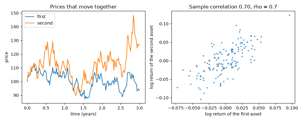
Over one frame the log return of each asset is its volatility times its Wiener increment plus a small drift, so the sample correlation of the two series of log returns should be close to rho, and their scatter should be an ellipse tilted along the diagonal.

trajectory = simulation.trajectory_
first, second = (np.diff(np.log(trajectory.values(f'{label}.price'))) for label in ('first', 'second'))
correlation = np.corrcoef(first, second)[0, 1]
fig, (paths, returns) = plt.subplots(1, 2, figsize=(10, 4))
paths.plot(trajectory.times, trajectory.values('first.price'), label='first')
paths.plot(trajectory.times, trajectory.values('second.price'), label='second')
paths.set_xlabel('time (years)')
paths.set_ylabel('price')
paths.set_title('Prices that move together')
paths.legend()
returns.scatter(first, second, s=6, alpha=0.6)
returns.set_xlabel('log return of the first asset')
returns.set_ylabel('log return of the second asset')
returns.set_title(f'Sample correlation {correlation:.2f}, rho = {RHO}')
fig.tight_layout()
plt.show()

Download Python source code: plot_correlated_geometric_brownian_motion.py

Download Jupyter notebook: plot_correlated_geometric_brownian_motion.ipynb

Gallery generated by mkdocs-gallery

About the model

Two assets whose prices follow geometric Brownian motions driven by correlated Wiener processes.

References

• Black and Scholes 1973
• Merton 1973