Note
Click here to download the full example code
Cubic autocatalysis
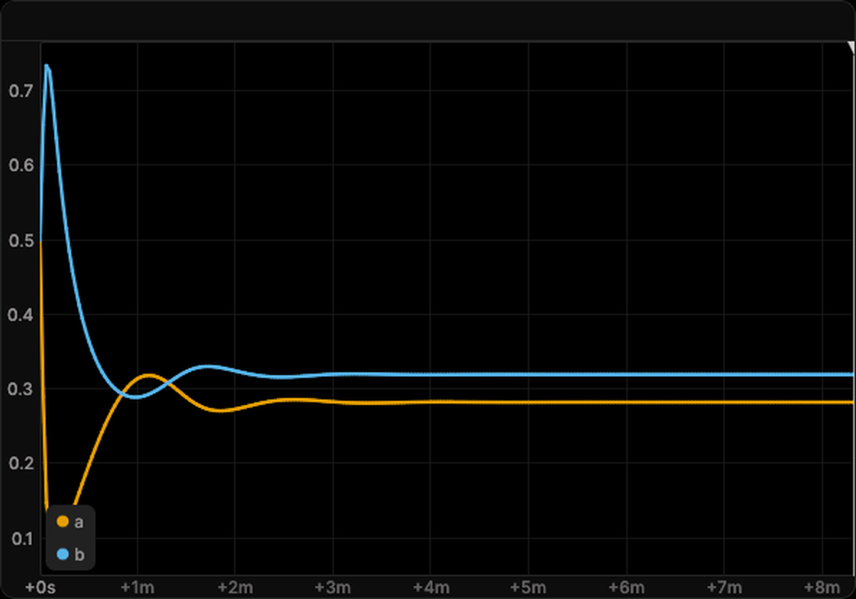
In a continuously fed reactor, the autocatalyst B either takes hold and keeps the reaction going, or is washed out.
Started with enough B, the reactor settles in the reacting state, where the reactant A stays low.
The model is created by name from the catalog with the feed rate F = 0.04 and the decay rate k = 0.05, for which
the washout state and a reacting state are both stable, and starts at a = b = 0.5. The default blueprint shows both
concentrations in one time series view.
import matplotlib.pyplot as plt
import numpy as np

from skcomplex.engine.runtime import Simulation
from skcomplex.engine.viz import RerunObserver
from skcomplex.models import create

MODEL = 'cubic_autocatalysis'

system = create(MODEL)
observer = RerunObserver(MODEL, save_path=f'{MODEL}.rrd', blueprint='default', interval=2)
simulation = Simulation(system, dt=1.0, observers=[observer]).check().prepare().run(until=500)
Open the recording in the Rerun viewer
Two basins of attraction
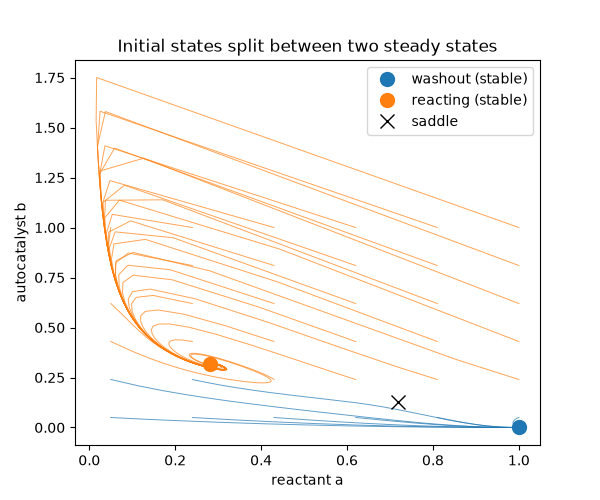
The steady states are the washout (1, 0) and the roots of (F + k) b^2 - F b + F (F + k) = 0 with
a = (F + k) / b: the larger root is a stable reacting state and the smaller one a saddle. Runs from a grid of
initial states should end in one of the two stable states, split by the separatrix through the saddle.
F, k = 0.04, 0.05
roots = np.roots([F + k, -F, F * (F + k)])
fig, ax = plt.subplots(figsize=(6, 5))
for a0 in np.linspace(0.05, 1.0, 6):
    for b0 in np.linspace(0.05, 1.0, 6):
        run = Simulation(create(MODEL, a=a0, b=b0, F=F, k=k), dt=2.0).check().prepare().run(until=800).trajectory_
        reacting = run.values('reactor.b')[-1] > 0.1
        ax.plot(
            run.values('reactor.a'),
            run.values('reactor.b'),
            color='C1' if reacting else 'C0',
            linewidth=0.7,
            alpha=0.7,
        )
ax.plot(1.0, 0.0, 'o', color='C0', markersize=10, label='washout (stable)')
ax.plot((F + k) / roots.max(), roots.max(), 'o', color='C1', markersize=10, label='reacting (stable)')
ax.plot((F + k) / roots.min(), roots.min(), 'x', color='black', markersize=10, label='saddle')
ax.set_xlabel('reactant a')
ax.set_ylabel('autocatalyst b')
ax.set_title('Initial states split between two steady states')
ax.legend()
plt.show()
About the model
Cubic autocatalysis A + 2B -> 3B with the decay B -> C in a continuously fed reactor.
References
- Gray and Scott 1983
- Trzaska 2023
Total running time of the script: ( 0 minutes 2.779 seconds)
Download Python source code: plot_cubic_autocatalysis.py