Note
Click here to download the full example code
Sample soccer data
This example shows SampleSoccerStats and SampleSoccerOdds, the sample data that ships with the library.
# Author: Georgios Douzas <gdouzas@icloud.com>
# Licence: MIT

import matplotlib.pyplot as plt

from sportsbet.dataloaders import DataLoader
from sportsbet.sources import SampleSoccerOdds, SampleSoccerStats
What the sample carries
It is a real season of the English and Spanish first divisions, taken from football-data.co.uk and frozen. It needs no key and reaches no network. That is why the examples and the tests use it.
stats = SampleSoccerStats()
stats.name, stats.kind, stats.sport
Out:
('sample_soccer', 'stats', 'soccer')
It ships with the library, so it knows what it publishes without reading anything.
stats.list_available_params()
Out:
[{'division': 1, 'league': 'England', 'year': 2024}, {'division': 1, 'league': 'Spain', 'year': 2024}]
Extracting the data
It is an ordinary source, so you use it like any other. Give it to a dataloader beside an odds source. Extracting reads the bundled files off your disk. That costs nothing and touches no network.
dataloader = DataLoader(param_grid={'league': ['England']}, stats=stats, odds=SampleSoccerOdds())
X_train, Y_train, O_train = dataloader.extract_train_data(odds_type='market_average')
The input data:
X_train
Out:
                            league  division  ...  away_points_avg home_points_avg
date                                          ...
2023-08-11 19:00:00+00:00  England         1  ...              NaN             NaN
2023-08-12 11:30:00+00:00  England         1  ...              NaN             NaN
2023-08-12 14:00:00+00:00  England         1  ...              NaN             NaN
2023-08-12 14:00:00+00:00  England         1  ...              NaN             NaN
2023-08-12 14:00:00+00:00  England         1  ...              NaN             NaN
...                            ...       ...  ...              ...             ...
2024-05-19 15:00:00+00:00  England         1  ...         1.837838        1.243243
2024-05-19 15:00:00+00:00  England         1  ...         1.243243        2.135135
2024-05-19 15:00:00+00:00  England         1  ...         1.189189        0.702703
2024-05-19 15:00:00+00:00  England         1  ...         1.405405        2.378378
2024-05-19 15:00:00+00:00  England         1  ...         1.702703        0.432432

[380 rows x 7 columns]
The multi-output targets:
Y_train
Out:
                           home_win__postplay__0min  ...  under_2.5__postplay__0min
date                                                 ...
2023-08-11 19:00:00+00:00                       0.0  ...                        0.0
2023-08-12 11:30:00+00:00                       1.0  ...                        0.0
2023-08-12 14:00:00+00:00                       0.0  ...                        1.0
2023-08-12 14:00:00+00:00                       1.0  ...                        0.0
2023-08-12 14:00:00+00:00                       0.0  ...                        1.0
...                                             ...  ...                        ...
2024-05-19 15:00:00+00:00                       1.0  ...                        0.0
2024-05-19 15:00:00+00:00                       1.0  ...                        1.0
2024-05-19 15:00:00+00:00                       0.0  ...                        0.0
2024-05-19 15:00:00+00:00                       1.0  ...                        0.0
2024-05-19 15:00:00+00:00                       0.0  ...                        0.0

[380 rows x 5 columns]
The odds:
O_train
Out:
                           market_average__away_win__preplay__0min  ...  market_average__under_2.5__preplay__0min
date                                                                ...
2023-08-11 19:00:00+00:00                                     1.35  ...                                      2.27
2023-08-12 11:30:00+00:00                                    15.67  ...                                      2.85
2023-08-12 14:00:00+00:00                                     2.64  ...                                      1.94
2023-08-12 14:00:00+00:00                                     9.61  ...                                      2.34
2023-08-12 14:00:00+00:00                                     3.30  ...                                      1.86
...                                                            ...  ...                                       ...
2024-05-19 15:00:00+00:00                                     3.67  ...                                      2.96
2024-05-19 15:00:00+00:00                                    14.55  ...                                      4.23
2024-05-19 15:00:00+00:00                                     2.23  ...                                      2.76
2024-05-19 15:00:00+00:00                                    21.81  ...                                      4.45
2024-05-19 15:00:00+00:00                                     1.35  ...                                      4.14

[380 rows x 5 columns]
It has no fixtures
The season is finished, so every match in it has been played. A fixture is a match that has not been played. The
sample has none, so extract_fixtures_data returns an empty frame with the training columns.
To bet on something, you need a source that is still publishing matches. See Football-Data. The sample is for learning the interface, not for betting.
X_fix, _, O_fix = dataloader.extract_fixtures_data()
len(X_fix)
Out:
0
A picture of it
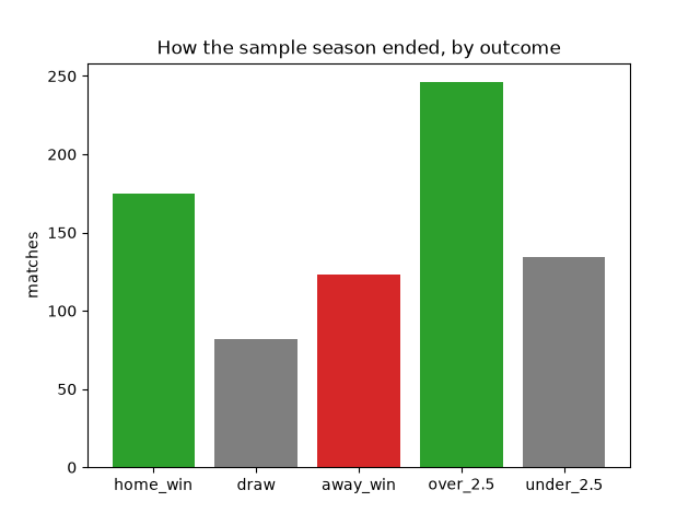
This shows how the season ended. Home wins lead. That lead is the home advantage the odds always price in.
outcomes = Y_train.sum()
outcomes.index = outcomes.index.str.split('__').str[0]

fig, ax = plt.subplots()
ax.bar(outcomes.index, outcomes.to_numpy(), color=['tab:green', 'tab:grey', 'tab:red'])
ax.set_title('How the sample season ended, by outcome')
ax.set_ylabel('matches')
Out:
Text(37.722222222222214, 0.5, 'matches')
Total running time of the script: ( 0 minutes 0.794 seconds)
Download Python source code: plot_sample_soccer.py