Note
Click here to download the full example code
Odds comparison bettor
This example shows OddsComparisonBettor. It bets by comparing the odds of different providers rather than by learning from the features.
# Author: Georgios Douzas <gdouzas@icloud.com>
# Licence: MIT

import matplotlib.pyplot as plt
import numpy as np
from sklearn.model_selection import TimeSeriesSplit

from sportsbet.dataloaders import DataLoader
from sportsbet.evaluation import OddsComparisonBettor, backtest
from sportsbet.sources import SampleSoccerOdds, SampleSoccerStats
Extracting the data
dataloader = DataLoader(
    param_grid={'league': ['England']},
    stats=SampleSoccerStats(),
    odds=SampleSoccerOdds(),
)
X_train, Y_train, O_train = dataloader.extract_train_data(odds_type='market_maximum')
A model that needs no features
It compares what one provider offers with what another offers. When the best price in the market is far enough above the average, the outcome is priced more generously than the market as a whole believes. That is the bet.
alpha sets how far above the average is far enough.
bettor = OddsComparisonBettor(alpha=0.03, betting_markets=['home_win', 'draw', 'away_win'])
_ = bettor.fit(X_train, Y_train, O_train)
These are the value bets, one boolean column per market. This bettor models the odds themselves, so it needs them at prediction time as well as at training time. A classifier bettor learns from the features alone.
bettor.bet(X_train, O_train)
Out:
array([[False, False,  True],
       [ True, False, False],
       [False, False,  True],
       ...,
       [False, False,  True],
       [ True, False, False],
       [False, False,  True]], shape=(380, 3))
Backtesting
results = backtest(bettor, X_train, Y_train, O_train, cv=TimeSeriesSplit(3))
results
Out:
                                                       Number of betting days  ...  Yield percentage per bet (away_win)
Training start Training end Testing start Testing end                          ...
2023-08-11     2023-10-28   2023-10-29    2023-12-30                       57  ...                                 -4.1
               2023-12-30   2023-12-30    2024-03-30                       66  ...                                  3.7
               2024-03-30   2024-03-30    2024-05-19                       56  ...                                  8.2

[3 rows x 11 columns]
Turning the one knob
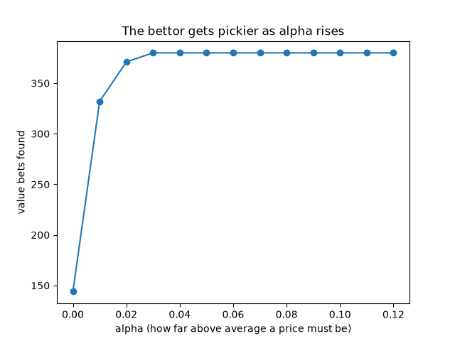
alpha is the whole model. A small alpha bets on almost every match and takes any price a little above the
average. A large alpha waits for the rare, clear mispricing. Sweep alpha and watch the bettor go from greedy to
picky.
alphas = np.linspace(0.0, 0.12, 13)
placed = []
for alpha in alphas:
    picky = OddsComparisonBettor(alpha=alpha, betting_markets=['home_win', 'draw', 'away_win'])
    picky.fit(X_train, Y_train, O_train)
    placed.append(int(picky.bet(X_train, O_train).sum()))

fig, ax = plt.subplots()
ax.plot(alphas, placed, marker='o')
ax.set_title('The bettor gets pickier as alpha rises')
ax.set_xlabel('alpha (how far above average a price must be)')
ax.set_ylabel('value bets found')
Out:
Text(37.722222222222214, 0.5, 'value bets found')
Total running time of the script: ( 0 minutes 2.767 seconds)
Download Python source code: plot_odds_comparison_bettor.py
Download Jupyter notebook: plot_odds_comparison_bettor.ipynb