Reinforcement Learning and LLM-based Agents

Leveraging Reinforcement Learning and LLMs for building smart, adaptive agents

Introduction

This presentation follows (Zhao 2025).

Reinforcement Learning

• An agent learns to optimize a specified target through trial and error interactions with the environment
• Traditional RL methods struggle with high-dimensional state spaces and complex environments
• Integration of deep learning techniques with RL has led to significant breakthroughs

Large Language Models

• LLMs typically refer to the Transformer-based language models containing hundreds of billions of parameters
• They tend to exhibit emergent abilities that are not present in small models
  • In-context learning
    • Task-related texts are included in the prompts as context information
  • Instruction following
    • Diverse task-specific datasets formatted with natural language descriptions
  • Step-by-step reasoning
    • Chain of Thought
    • Tree of Thought
    • Graph of Thought

LLM-enhanced Reinforcement Learning

• Methods that utilize the high-level cognitive capabilities of pre-trained LLM models to assist the RL paradigm
• Taxonomy
  • Information processor
    • Feature representations extraction
    • Information translation to DSL
  • Reward designer
    • Implicit
    • Explicit
  • Decision-maker
    • Action making
    • Action guiding
  • Generator
    • World model simulator
    • Policy interpreter

Introduction to Markov Decision Process

Description

A Markov Decision Process is a mathematical framework used to describe decision-making in situations where outcomes are partly random and partly controlled by an agent.

At each time step, the agent:

• Observes the current state of the environment
• Takes an action, which may lead to a transition to a new state
• Receives a reward based on the action taken and the resulting state

The goal of the agent is to maximize the cumulative reward over time by choosing the best possible actions based on the current state.

Autonomous driving

• State space: \(\mathscr{S} = \left\{ (\text{position}, \text{speed}, \text{lane}, \text{proximity to vehicles}, \text{traffic signals})_1, \dots \right\}\)
• Action space: \(\mathscr{A} = \{ \text{accelerate}, \text{brake}, \text{left}, \text{right}, \text{stay} \}\)
• Reward space: \(\mathscr{R} = \{ \text{+1 for safe driving}, \text{-10 for collision}, \text{+5 for reaching the goal} \}\)
• Model: The dynamics describe the effects of the vehicle’s actions on its next state, such as how acceleration changes speed and position.

Healthcare treatment planning

• State Space: \(\mathscr{S} = \left\{ \big(\text{disease state}, \text{treatment response}, \text{vital signs}, \text{age} \big)_1, \dots \right\}\)
• Action Space: \(\mathscr{A} = \{ \text{drug A}, \text{drug B}, \text{surgery}, \text{no treatment} \}\)
• Reward Space: \(\mathscr{R} = \{ \text{+10 for recovery}, \text{-5 for side effects}, \text{-10 for relapse} \}\)
• Model: The dynamics describe how treatments affect the patient’s health, with probabilistic transitions between health states based on treatment and health conditions.

Probability Theory

Random experiment

A Random experiment is a process that produces an unpredictable outcome.

Example

A rolling a fair die.

Probability space

A probability space \((S, F, P)\) is defined as follows:

• Sample space \(S\)
  • Set of possible outcomes
• Sigma-algebra \(F\)
  • \(A \in F \Rightarrow A^c \in F\)
  • \(\{A_i\}_{i=1}^{\infty} \subseteq F \Rightarrow \bigcup_{i=1}^{\infty} A_i \in F\)
• Probability measure \(P\)
  • \(P: F \rightarrow \mathbb{R}\)
    • Non-negativity \(P(A) \geq 0\) for all \(A \in F\)
    • Normalization \(P(S) = 1\)
    • Countable additivity \(P\left(\bigcup_{i=1}^{\infty} A_i\right) = \sum_{i=1}^{\infty} P(A_i)\), \(A_i\) disjoint

Example

• Sample space \(S\)
  • \(S = \{1, 2, 3, 4, 5, 6\}\)
• Sigma-algebra \(F\)
  • \(F = \{\emptyset, \{1\}, \{2\}, \dots, S\}\)
• Probability measure \(P\)
  • \(P(\{i\}) = \frac{1}{6}\) for each \(i \in S\)

Random variable

A random variable \(X\) is a function \(X: S \to \mathbb{R}\) such that \(\forall x \in \mathbb{R}\):

\[X^{-1}((-\infty, x]) \in F\]

Example

• \(X(s) = s\)
• \(Y(s) = \begin{cases} 1, & \text{if } s \text{ is even} \\ 0, & \text{if } s \text{ is odd} \end{cases}\)
• \(Z(s) = \begin{cases} 1, & \text{if } s \leq 3 \\ 0, & \text{if } s > 3 \end{cases}\)

PMF

The PMF of a discrete random variable \(X\) is a function \(p_X: \mathbb{R} \to [0, 1]\) such that:

\[p_X(x) = P(X = x)\]

Example

• \(p_X(x) = \frac{1}{6}\) for \(x = 1, 2, 3, 4, 5, 6\)
• \(p_Y(0) = p_Y(1) = \frac{3}{6} = 0.5\)
• \(p_Z(0) = p_Z(1) = \frac{3}{6} = 0.5\)

Joint PMF

The joint PMF of two discrete random variables \(X\) and \(Y\) is defined as follows:

\[p_{X,Y}(x, y) = P(X = x, Y = y)\]

Example

• \(p_{X,Y}(x, y) =\begin{cases} \frac{1}{6}, & \text{if } (x, y) \in \{(1, 0), (2, 1), (3, 0), (4, 1), (5, 0), (6, 1)\} \\ 0, & \text{otherwise} \end{cases}\)

Conditional PMF

The conditional PMF of two discrete random variables \(X\) and \(Y\) is defined as follows:

\[p_{Y|X}(y | x) = \frac{P_{X,Y}(x, y)}{P_X(x)}\]

Example

• \(p_{Y|X}(y | x=2) = \begin{cases} 1, & \text{if } y = 1 \\ 0, & \text{if } y = 0 \end{cases}\)

Independence

Two random variables \(X\) and \(Y\) are independent when for all \(x, y\) the following condition holds:

\[p_{X,Y}(x, y) = P_X(x)P_Y(y)\]

Example

• \(p_{X,Y}(x, y) \neq p_X(x)p_Y(y)\) and \(X\), \(Y\) are not independent

Conditional independence

Two random variables \(X\) and \(Y\) are conditionally independent given the random variable \(Z\) when for all \(x, y, z\) the following condition holds:

\[p_{Y|X, Z}(y | x, z) = P_{Y|Z}(y | z)\]

Example

• \(p_{Y|X,Z}(y | x, z) = p_{Y|X}(y | x) = \begin{cases} 1, & \text{if } x \text{ is even and } y = 1 \\ 1, & \text{if } x \text{ is odd and } y = 0 \\ 0, & \text{otherwise} \end{cases}\)

Joint PMF law of total probability

The joint PMF of two random variables \(X\) and \(Y\) satisfies the following relation:

\[p_X(x) = \sum_y p_{X, Y}(x, y)\]

Example

• \(\sum_y p_{X, Y}(x, y) = p_{X, Y}(x, 0) + p_{X, Y}(x, 1) = p_X(x)\)
• \(\sum_x p_{X, Y}(x, y) = p_{X, Y}(1, y) + p_{X, Y}(2, y) + \cdots = p_Y(y)\)

Conditional PMF chain rule

The chain rule of conditional PMFs is the following:

\[p_{X|Y}(x \mid y)=\sum_z p_{X|Z,Y}(x \mid z, y) p_{Z|Y}(z \mid y)\]

Example

• \(p_{X|Z,Y}(x \mid z, y) =\begin{cases} \frac{1}{2}, & \text{if } x = 4 \text{ or } 6, z = 1, y = 1 \\ 1, & \text{if } x = 2, z = 0, y = 1 \\ 1, & \text{if } x = 5, z = 1, y = 0 \\ \frac{1}{2}, & \text{if } x = 1 \text{ or } 3, z = 0, y = 0 \\ 0, & \text{otherwise} \end{cases}\)
• \(p_{Z|Y}(z \mid y) = \begin{cases} \frac{2}{3}, & \text{if } z = 1 \text{ and } y = 1 \\ \frac{1}{3}, & \text{if } z = 0 \text{ and } y = 1 \\ \frac{1}{3}, & \text{if } z = 1 \text{ and } y = 0 \\ \frac{2}{3}, & \text{if } z = 0 \text{ and } y = 0 \\0, & \text{otherwise} \end{cases}\)
• \(p_{X|Y}(x \mid y) = \begin{cases} \frac{1}{3}, & \text{if } x \text{ is even and } y = 1 \\ \frac{1}{3}, & \text{if } x \text{ is odd and } y = 0 \\ 0, & \text{otherwise} \end{cases}\)

Expectation

The expectation of a discrete random variable \(X\) is defined as follows:

\[\mathbb{E}[X]=\sum_x p_X(x) x\]

Example

• \(\mathbb{E}[X]= (1 + 2 + 3 + 4 + 5 + 6) \cdot \frac{1}{6} = 3.5\)

Conditional expectation

The conditional expectation of two discrete random variables \(X\) and \(Y\) is defined as follows:

\[\mathbb{E}[X \mid Y=y]=\sum_x x p_{X|Y}(x \mid y)\]

Example

• \(\mathbb{E}[X \mid Y=1] = \sum_x x p_{X|Y}(x \mid y=1) = (2 + 4 + 6) \cdot \frac{1}{3} = 4\)

Law of total expectation

The law of total expectation of two discrete random variables \(X\) and \(Y\) is the following:

\[\mathbb{E}[X]=\sum_y \mathbb{E}[X \mid Y=y] p_Y(y)\]

Example

• \(\mathbb{E}[X]= \mathbb{E}[X \mid Y=1] p_Y(1) + \mathbb{E}[X \mid Y=0] p_Y(0) = \frac{4 + 3}{2} = 3.5\)

Variance

The variance of a random variable \(X\) is defined as follows:

\[\operatorname{var}(X)=\mathbb{E}\left[(X-\bar{X})^2\right] = \mathbb{E}[X^2] - (\mathbb{E}[X])^2\]

Example

• \(\operatorname{var}(X) = \frac{1^2 + \cdots + 6^2}{6} - 3.5^2 \approx 2.92\)

Covariance

The covariance of two random variables \(X\) and \(Y\) is defined as follows:

\[\operatorname{cov}(X, Y)=\mathbb{E}[(X-\bar{X})(Y-\bar{Y})] = \mathbb{E}[XY] - \mathbb{E}[X] \mathbb{E}[Y]\]

Example

• \(\operatorname{cov}(X, Y)=\sum_{x,y} p_{X, Y}(x, y) xy - \mathbb{E}[X] \mathbb{E}[Y] = 0.25\)

Covariance matrix

The covariance of a random vector \(\vec{X}\) is defined as follows:

\[\Sigma=\mathbb{E} \left[(\vec{X}- \bar{\vec{X}})(\vec{X}-\bar{\vec{X}})^T\right] \in \mathbb{R}^{n \times n}\]

In components form:

\[[\Sigma]_{i j} = \operatorname{cov}\left(X_i, X_j\right)\]

Example

• \(\Sigma = \begin{pmatrix} \text{Var}(X) & \text{Cov}(X, Y) & \text{Cov}(X, Z) \\ \text{Cov}(Y, X) & \text{Var}(Y) & \text{Cov}(Y, Z) \\ \text{Cov}(Z, X) & \text{Cov}(Z, Y) & \text{Var}(Z) \end{pmatrix} = \begin{pmatrix} 2.92 & 0.25 & -0.75 \\ 0.25 & 0.25 & \frac{1}{12} \\ -0.75 & \frac{1}{12} & 0.25 \end{pmatrix}\)

Basics of Markov Decision Process

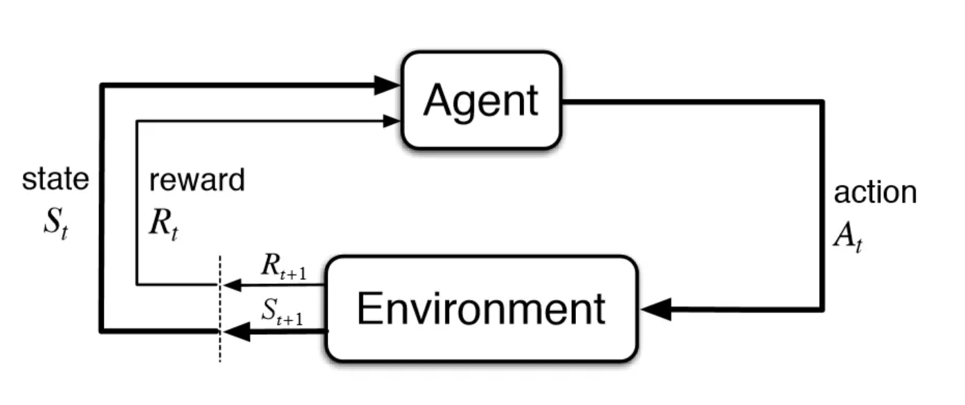
Definition

• Sets
  • State space: \(\mathscr{S}=\left\{s_1, s_2, \ldots \right\}\)
  • Action space: \(\mathscr{A}(s)=\left\{a_1, a_2, \ldots, \right\}\)
  • Reward space: \(\mathscr{R}(s, a)=\left\{r_1, r_2, \ldots \right\}\)
• Model
  • State transition: \(p(s' \mid s, a)\)
  • Reward: \(p(r \mid s, a)\)
• Policy
  • \(\pi(a \mid s) = p(a \mid s)\)
• Markov property
  • \(p\left(s_{t+1} \mid s_t, a_t, s_{t-1}, \ldots \right)=p\left(s_{t+1} \mid s_t, a_t\right)\)
  • \(p\left(r_{t+1} \mid s_t, a_t, s_{t-1}, \ldots \right)=p\left(r_{t+1} \mid s_t, a_t\right)\)

Example

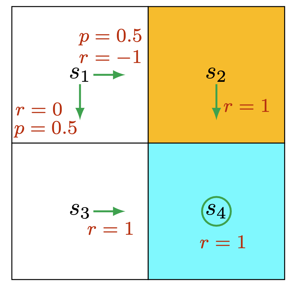
• Sets
  • State space: \(\mathscr{S} = \{ s_1, s_2, s_3, s_4 \}\)
  • Action space: \(\mathscr{A} = \{ \uparrow, \downarrow, \leftarrow, \rightarrow, \bigcirc \}\)
  • Reward space: \(\mathscr{R} = \{ -1, +1, 0 \}\)
• Model
  • State transition: \(p(s' \mid s, a) = 0 \text{ or } 1\)
  • Reward: \(p(r \mid s, a) = 0 \text{ or } 1\)
• Policy
  • \(\pi(a \mid s) = 0 \text{ or } 1\)
• Markov property
  • \(p\left(s_{t+1} \mid s_t, a_t, s_{t-1}, \ldots \right)=p\left(s_{t+1} \mid s_t, a_t\right)\)
  • \(p\left(r_{t+1} \mid s_t, a_t, s_{t-1}, \ldots \right)=p\left(r_{t+1} \mid s_t, a_t\right)\)

State-action-reward trajectory

The state-action-reward trajectory is defined as follows:

\[\ldots S_t, R_{t} \overset{A_t} \rightarrow S_{t+1}, R_{t+1} \overset{A_{t+1}} \rightarrow S_{t+2}, R_{t+2} \ldots\]

Example

• \(\ldots s_1, 0 \overset{\downarrow} \rightarrow s_3, 0 \overset{\rightarrow} \rightarrow s_4, 1 \overset{\bigcirc} \rightarrow s_4, 1 \overset{\bigcirc} \rightarrow \ldots\)

Discounted return

The discounted return is defined as follows:

\[G_t = R_{t+1} + \gamma \cdot R_{t+2} + \gamma^2 \cdot R_{t+3} + \cdots\]

Example

• \(G_t = 0 + \gamma \cdot 1 + \gamma^2 \cdot 1 + \cdots = \frac{\gamma}{1-\gamma}\)

Terminal state

• Exists \(s_{T}\) that resets the next state to a starting state
  • Episodic task: There are terminal states
  • Continuing task: There are no terminal states

Example

State Value and Bellman Equation

State value

The state value is defined as follows:

\[v_\pi(s) \doteq \mathbb{E}\left[G_t \mid S_t=s\right]\]

Example

• \(v_\pi(s_1) = -0.5 + \frac{\gamma}{1-\gamma}\)
• \(v_\pi(s_2) = \frac{1}{1-\gamma}\)
• \(v_\pi(s_3) = \frac{1}{1-\gamma}\)
• \(v_\pi(s_4) = \frac{1}{1-\gamma}\)

Bellman equation

The Bellman equation of the state values is the following:

\[v_\pi(s) = \sum_{a \in \mathscr{A}} \pi(a \mid s)\left[\sum_{r \in \mathscr{R}} p(r \mid s, a) r+\gamma \sum_{s^{\prime} \in \mathscr{S}} p\left(s^{\prime} \mid s, a\right) v_\pi\left(s^{\prime}\right)\right]\]

Example

• \(v_\pi(s_1) = -0.5 + 0.5 \gamma (v_\pi(s_2) + v_\pi(s_3))\)
• \(v_\pi(s_2) = 1 + \gamma v_\pi(s_4)\)
• \(v_\pi(s_3) = 1 + \gamma v_\pi(s_4)\)
• \(v_\pi(s_4) = 1 + \gamma v_\pi(s_4)\)

Bellman equation equivalent forms

The Bellman equation can be written as follows:

\[v_\pi(s)=\sum_{a \in \mathscr{A}} \pi(a \mid s) \sum_{s^{\prime} \in \mathscr{S}} \sum_{r \in \mathscr{R}} p\left(s^{\prime}, r \mid s, a\right)\left[r+\gamma v_\pi\left(s^{\prime}\right)\right]\]

If the reward depends only on the next state the Bellman equation can be written as follows:

\[v_\pi(s)=\sum_{a \in \mathscr{A}} \pi(a \mid s) \sum_{s^{\prime} \in \mathscr{S}} p\left(s^{\prime} \mid s, a\right)\left[r\left(s^{\prime}\right)+\gamma v_\pi\left(s^{\prime}\right)\right]\]

Bellman equation matrix-vector form

The Bellman equation in matrix vector form is written as follows:

\[v_\pi=r_\pi+\gamma P_\pi v_\pi\]

where

\[\left[r_\pi\right]_s \doteq \sum_{a \in \mathscr{A}} \pi(a \mid s) \sum_{r \in \mathscr{R}} p(r \mid s, a) r\]

\[\left[P_\pi\right]_{s s^{\prime}} \doteq \sum_{a \in \mathscr{A}} \pi(a \mid s) p\left(s^{\prime} \mid s, a\right)\]

The state transition matrix \(P\) has the following properties:

\[P_\pi \geq 0\]

\[P_\pi \mathbf{1}=\mathbf{1}\]

\[\exists (I-\gamma P_\pi)^{-1}\]

\[\left(I-\gamma P_\pi\right)^{-1} \geq I\]

\[\left(I-\gamma P_\pi\right)^{-1} r \geq , r \geq 0\]

\[\left(I-\gamma P_\pi\right)^{-1} r_1 \geq\left(I-\gamma P_\pi\right)^{-1} r_2, r_1 \geq r_2\]

Example

• \(r_\pi = \left[\begin{array}{c}0.5(0)+0.5(-1) \\ 1 \\ 1 \\ 1\end{array}\right]\)
• \(P_\pi = \left[\begin{array}{cccc}0 & 0.5 & 0.5 & 0 \\ 0 & 0 & 0 & 1 \\ 0 & 0 & 0 & 1 \\ 0 & 0 & 0 & 1\end{array}\right]\)

Policies and state values

Example

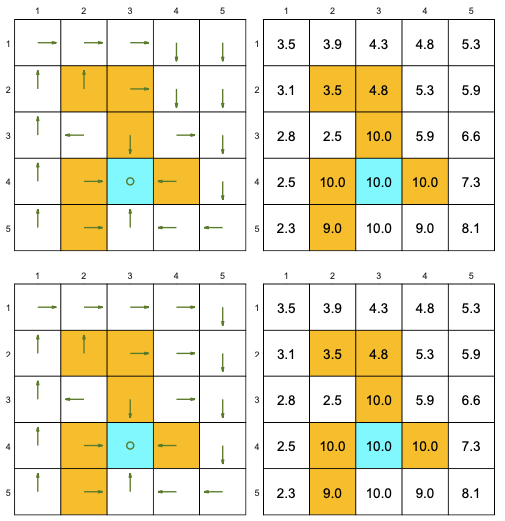
The following “good” policies are different but they have the same state values:

Example

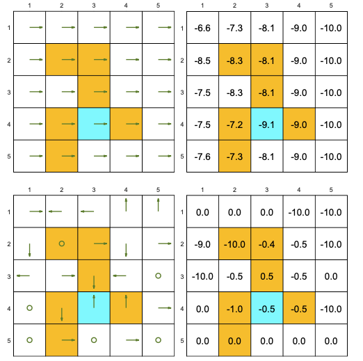
The following “bad” policies have lower state values:

Bellman equation closed-form solution

\[v_\pi=\left(I-\gamma P_\pi\right)^{-1} r_\pi\]

Bellman equation iterative solution

\[v_{k+1}=r_\pi+\gamma P_\pi v_k, \quad k=0,1,2, \ldots\]

State transition probability

\[[P]_{(s, a), s^{\prime}}=p\left(s^{\prime} \mid s, a\right)\]

import numpy as np
P = np.array(
    [
        [1., 0., 0., 0.],
        [0., 0., 1., 0.],
        [1., 0., 0., 0.],
        [0., 1., 0., 0.],
        [1., 0., 0., 0.],
        [0., 1., 0., 0.],
        [0., 0., 0., 1.],
        [1., 0., 0., 0.],
        [0., 1., 0., 0.],
        [0., 1., 0., 0.],
        [1., 0., 0., 0.],
        [0., 0., 1., 0.],
        [0., 0., 1., 0.],
        [0., 0., 0., 1.],
        [0., 0., 1., 0.],
        [0., 1., 0., 0.],
        [0., 0., 0., 1.],
        [0., 0., 1., 0.],
        [0., 0., 0., 1.],
        [0., 0., 0., 1.]
    ]
)

Reward probability

\[[R]_{(s, a), r}=p\left(r \mid s, a\right)\]

R = np.array(
    [
        [1., 0., 0.],
        [0., 0., 1.],
        [1., 0., 0.],
        [1., 0., 0.],
        [0., 0., 1.],
        [1., 0., 0.],
        [0., 1., 0.],
        [0., 0., 1.],
        [1., 0., 0.],
        [1., 0., 0.],
        [0., 0., 1.],
        [1., 0., 0.],
        [1., 0., 0.],
        [0., 1., 0.],
        [0., 0., 1.],
        [1., 0., 0.],
        [1., 0., 0.],
        [0., 0., 1.],
        [1., 0., 0.],
        [0., 1., 0.]
    ]
)

Policy probability

\[[\Pi]_{a, s} = p(a \mid s)\]

Pi = np.array([
    [0.0, 0.0, 0.0, 0.0],
    [0.5, 1.0, 0.0, 0.0],
    [0.0, 0.0, 0.0, 0.0],
    [0.5, 0.0, 1.0, 0.0],
    [0.0, 0.0, 0.0, 1.0]
])

Expected reward under policy

\[\left[r_\pi\right]_s = \sum_{a \in \mathscr{A}} \pi(a \mid s) \sum_{r \in \mathscr{R}} p(r \mid s, a) r\]

\[\left[r_\pi\right]_s = \sum_{a \in \mathscr{A}} \big( R \cdot \left[\begin{array}{c}-1 & 1 & 0 \end{array}\right]^T \big)_{s, a} \cdot [\Pi]_{a, s}\]

r_space = np.array([-1, 1, 0])
r_p = np.diagonal(
    np.matmul(
        np.dot(R, r_space).reshape(4, 5), 
        Pi
    )
)
r_p

array([-0.5,  1. ,  1. ,  1. ])

State transition probability under policy

\[\left[P_\pi\right]_{s s^{\prime}} = \sum_{a \in \mathscr{A}} \pi(a \mid s) p\left(s^{\prime} \mid s, a\right)\]

\[\left[P_\pi\right]_{s s^{\prime}} = \sum_{a \in \mathscr{A}} [\Pi^T]_{s, a} [P]_{(s, a), s^{\prime}}\]

P_p = np.diagonal(
    np.matmul(
        P.T.reshape(4,4,5), 
        Pi
    ).T
).T
P_p

array([[0. , 0.5, 0.5, 0. ],
       [0. , 0. , 0. , 1. ],
       [0. , 0. , 0. , 1. ],
       [0. , 0. , 0. , 1. ]])

Implementing Bellman equation closed-form solution

\[v_\pi=\left(I-\gamma P_\pi\right)^{-1} r_\pi\]

gamma = 0.9
I = np.identity(r_p.size)
v_cfs = np.dot(np.linalg.inv(I - gamma * P_p), r_p)
v_cfs

array([ 8.5, 10. , 10. , 10. ])

Implementing Bellman equation iterative solution

\[v_{k+1}=r_\pi+\gamma P_\pi v_k, \quad k=0,1,2, \ldots\]

tol = 1e-5
v_is = np.zeros_like(r_p)
while True:
    v_is_current = v_is
    v_is = r_p + gamma * np.dot(P_p, v_is)
    diff = np.abs(v_is - v_is_current)
    if np.any(diff < tol):
        break
v_is

array([8.49991665, 9.99991665, 9.99991665, 9.99991665])

Action Value and Bellman Equation

Action value

The action value is defined as follows:

\[q_\pi(s, a) \doteq \mathbb{E}\left[G_t \mid S_t=s, A_t=a\right]\]

Example

• \(q_\pi(s_1, \rightarrow) = -1 + \gamma \frac{1}{1-\gamma}\)
• \(q_\pi(s_1, \downarrow) = \gamma \frac{1}{1-\gamma}\)
• \(q_\pi(s_1, \leftarrow) = -1 + \gamma (-0.5 + \frac{\gamma}{1-\gamma})\)
• \(q_\pi(s_1, \uparrow) = -1 + \gamma (-0.5 + \frac{\gamma}{1-\gamma})\)
• \(q_\pi(s_1, \bigcirc) = \gamma (-0.5 + \frac{\gamma}{1-\gamma})\)
• \(q_\pi(s_2, \rightarrow) = -1 + \gamma \frac{1}{1-\gamma}\)
• \(q_\pi(s_2, \downarrow) = 1 + -1 + \gamma \frac{1}{1-\gamma}\)
• \(q_\pi(s_2, \leftarrow) = \gamma (-0.5 + \frac{\gamma}{1-\gamma})\)
• \(q_\pi(s_2, \uparrow) = -1 + \gamma \frac{1}{1-\gamma}\)
• \(q_\pi(s_2, \bigcirc) = -1 + \gamma \frac{1}{1-\gamma}\)
• \(q_\pi(s_3, \rightarrow) = 1 + \gamma \frac{1}{1-\gamma}\)
• \(q_\pi(s_3, \downarrow) = -1 + \gamma \frac{1}{1-\gamma}\)
• \(q_\pi(s_3, \leftarrow) = -1 + \gamma \frac{1}{1-\gamma}\)
• \(q_\pi(s_3, \uparrow) = 1 + \gamma (-0.5 + \frac{\gamma}{1-\gamma})\)
• \(q_\pi(s_3, \bigcirc) = \gamma \frac{1}{1-\gamma}\)
• \(q_\pi(s_4, \rightarrow) = -1 + \gamma \frac{1}{1-\gamma}\)
• \(q_\pi(s_4, \downarrow) = -1 + \gamma \frac{1}{1-\gamma}\)
• \(q_\pi(s_4, \leftarrow) = \gamma \frac{1}{1-\gamma}\)
• \(q_\pi(s_4, \uparrow) = -1 + \gamma \frac{1}{1-\gamma}\)
• \(q_\pi(s_4, \bigcirc) = 1 + \gamma \frac{1}{1-\gamma}\)

Action value to state value

The following formula provides the conversion from action to state value:

\[v_\pi(s)=\sum_{a \in \mathscr{A}} \pi(a \mid s) q_\pi(s, a)\]

Example

• \(v_\pi(s_1) = 0.5 + 0.5 \gamma \frac{1}{1-\gamma} = -0.5 + \frac{\gamma}{1-\gamma}\)

State value to action value

The following formula provides the conversion from state to action value:

• \(q_\pi(s, a)=\sum_{r \in \mathscr{R}} p(r \mid s, a) r+\gamma \sum_{s^{\prime} \in \mathscr{S}} p\left(s^{\prime} \mid s, a\right) v_\pi\left(s^{\prime}\right)\)

Example

• \(q_\pi(s_1, \rightarrow) = 1(-1) + \gamma v_\pi(s_2) = -1 + \gamma \frac{1}{1-\gamma}\)

Bellman equations

The Bellman equation of the action values is the following:

\[q_\pi(s, a)=\sum_{r \in \mathscr{R}} p(r \mid s, a) r+\gamma \sum_{s^{\prime} \in \mathscr{S}} p\left(s^{\prime} \mid s, a\right) \sum_{a^{\prime} \in \mathscr{A}\left(s^{\prime}\right)} \pi\left(a^{\prime} \mid s^{\prime}\right) q_\pi\left(s^{\prime}, a^{\prime}\right)\]

Example

• \(q_\pi(s_1, \rightarrow) = -1 + \gamma q_\pi(s_2, \downarrow)\)
• \(q_\pi(s_1, \downarrow) = \gamma q_\pi(s_3, \rightarrow)\)
• \(q_\pi(s_1, \leftarrow) = -1 + \gamma (q_\pi(s_1, \rightarrow) + q_\pi(s_1, \downarrow))\)
• \(q_\pi(s_1, \uparrow) = -1 + \gamma (q_\pi(s_1, \rightarrow) + q_\pi(s_1, \downarrow))\)
• \(q_\pi(s_1, \bigcirc) = \gamma (q_\pi(s_1, \rightarrow) + q_\pi(s_1, \downarrow))\)
• \(q_\pi(s_2, \rightarrow) = -1 + \gamma q_\pi(s_2, \downarrow)\)
• \(q_\pi(s_2, \downarrow) = 1 + + \gamma q_\pi(s_4, \bigcirc)\)
• \(q_\pi(s_2, \leftarrow) = \gamma (q_\pi(s_1, \rightarrow) + q_\pi(s_4, \downarrow))\)
• \(q_\pi(s_2, \uparrow) = -1 + \gamma q_\pi(s_2, \downarrow)\)
• \(q_\pi(s_2, \bigcirc) = -1 + \gamma q_\pi(s_2, \downarrow)\)
• \(q_\pi(s_3, \rightarrow) = 1 + \gamma q_\pi(s_4, \bigcirc)\)
• \(q_\pi(s_3, \downarrow) = -1 + \gamma q_\pi(s_3, \rightarrow)\)
• \(q_\pi(s_3, \leftarrow) = -1 + \gamma q_\pi(s_3, \rightarrow)\)
• \(q_\pi(s_3, \uparrow) = 1 + \gamma (q_\pi(s_1, \rightarrow) + q_\pi(s_1, \downarrow))\)
• \(q_\pi(s_3, \bigcirc) = \gamma q_\pi(s_3, \rightarrow)\)
• \(q_\pi(s_4, \rightarrow) = -1 + \gamma q_\pi(s_4, \bigcirc)\)
• \(q_\pi(s_4, \downarrow) = -1 + \gamma q_\pi(s_4, \bigcirc)\)
• \(q_\pi(s_4, \leftarrow) = \gamma q_\pi(s_3, \rightarrow)\)
• \(q_\pi(s_4, \uparrow) = -1 + \gamma q_\pi(s_2, \downarrow)\)
• \(q_\pi(s_4, \bigcirc) = 1 + \gamma q_\pi(s_4, \bigcirc)\)

Bellman equation matrix-vector form

The Bellman equation in matrix vector form is written as follows:

\[q_\pi=\tilde{r}+\gamma P \Pi q_\pi\]

where

\[\left[q_\pi\right]_{(s, a)}=q_\pi(s, a)\]

\[[\tilde{r}]_{(s, a)}=\sum_{r \in \mathscr{R}} p(r \mid s, a) r\]

\[[P]_{(s, a), s^{\prime}}=p\left(s^{\prime} \mid s, a\right)\]

\[\Pi_{s^{\prime},\left(s^{\prime}, a^{\prime}\right)}=\pi\left(a^{\prime} \mid s^{\prime}\right)\]

Example

• \(\tilde{r} = \left[\begin{array}{c} -1 \\ 0 \\ -1 \\ -1 \\ 0 \\ \vdots\end{array}\right]\)
• \(P = \left[\begin{array}{cccc}1 & 0 & 0 & 0 \\ 0 & 0 & 1 & 0 \\ 1 & 0 & 0 & 0 \\ 0 & 1 & 0 & 0 \\ 1 & 0 & 0 & 0 \\ \vdots & \vdots & \vdots & \vdots \end{array}\right]\)
• \(\Pi = \left[\begin{array}{cccc}0 & 0.5 & 0 & 0.5 & 0 & 0 & 0 & 0 & 0 & 0 &\dots \\ 0 & 0 & 0 & 0 & 0 & 0 & 1 & 0 & 0 & 0 &\dots \\ 0 & 0 & 0 & 0 & 0 & 0 & 0 & 0 & 0 & 0 & \dots \\ 0 & 0 & 0 & 0 & 0 & 0 & 0 & 0 & 0 & 0 & \dots \end{array}\right]\)

References

Zhao, Shiyu. 2025. Mathematical Foundations of Reinforcement Learning. Springer Nature Singapore. https://doi.org/10.1007/978-981-97-3944-8.