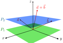
Physical space

Introduction
It’s quite common to think of physical space as \(\mathbb{R}^3\), but this perspective can be misleading, both from a mathematical and a physical standpoint. Instead, the three-dimensional space we encounter in Classical Physics (and even the four-dimensional spacetime in Special Relativity) is more accurately captured by the concept of affine spaces.
Definition
To understand this better, let’s dive into what a real affine space is. A real affine space of finite dimension \(n\), denoted by \(\mathbb{A}^n\), is a collection of elements known as points, but with some additional structure:
- There’s an associated \(n\)-dimensional vector space \(V\), which we call the space of displacements or the space of free vectors.
- A mapping \(\mathbb{A}^n \times \mathbb{A}^n \ni (P, Q) \mapsto P - Q \in V\) that respects certain conditions:
- For every point \(Q\in \mathbb{A}^n\) and every vector \(\mathbf{v} \in V\), there’s a unique point \(P \in \mathbb{A}^n\) such that \(P - Q =\mathbf{v}\).
- For any three points \(P, Q, R \in \mathbb{A}^n\), the equation \(P - Q + Q - R = P - R\) always holds.
Example
A trivial example is the real affine space \(\mathbb{A}^n = \mathbb{R}^n\) with the displacement space being the vector space \(\mathbb{R}^n\). A more interesting example is the system \(\begin{cases}x + y + z = 2 \\2x + y - z = 1\end{cases}\)
The solution space of the system is an affine space \(\mathbb{A}^3\):
Matplotlib is building the font cache; this may take a moment.Additionally, the the solution space of the homogeneous system is the space of displacements \(V\):
We can get a particular solution \(Q \in \mathbb{A}^3\) and verify that it is indeed a solution:
The general solution of the system is given by the displacement of \(Q\). For example another solution \(P \in \mathbb{A}^3\) is the following: